IMF API with Python: Practical Examples
Parts 1 and 2 covered the basics of retrieving data and discovering datasets. Here we apply both—combining the discovery tools from Part 2 with practical workflows—to work through three examples: economic forecasts, commodity prices, and bulk downloads.
Economic Forecasts (WEO)
The World Economic Outlook (WEO) dataset contains IMF projections for over 40 indicators—GDP, inflation, unemployment, government debt, current account, and more—covering nearly every country. Data includes historical values and forecasts several years forward.
In[1]:
import sdmx
import pandas as pd
import matplotlib.pyplot as plt
import logging
logging.getLogger('sdmx').setLevel(logging.ERROR)

IMF_DATA = sdmx.Client('IMF_DATA')
We can use the discovery methods from Part 2 to explore the WEO dataset and find the right indicator code. Here we look at the dataset's dimensions and search for GDP-related indicators:
In[2]:
# Explore WEO structure (Part 2 techniques)
f = IMF_DATA.dataflow('WEO')
dsd = list(f.structure.values())[0]
print('Dimensions:', [d.id for d in dsd.dimensions.components])

# Search for GDP growth indicators
for name, cl in f.codelist.items():
    codes = sdmx.to_pandas(cl)
    matches = codes[codes.str.contains('GDP.*constant', case=False)]
    if not matches.empty:
        print(f'\n{matches}')
Out[2]:
Dimensions: ['COUNTRY', 'INDICATOR', 'FREQUENCY', 'TIME_PERIOD']

INDICATOR
NGDP_R       Gross domestic product, constant prices (National currency)
NGDP_RPCH    Gross domestic product, constant prices (Percent change)
Name: ..., dtype: object
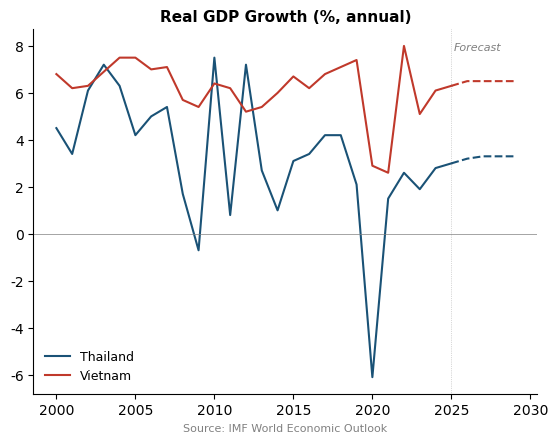
The indicator we want is NGDP_RPCH—annual percent change in real GDP. Let's compare Thailand and Vietnam, two fast-growing Southeast Asian economies:
In[3]:
# Real GDP growth: Thailand vs. Vietnam
key = 'THA+VNM.NGDP_RPCH.A'
data_msg = IMF_DATA.data('WEO', key=key)

df = sdmx.to_pandas(data_msg).reset_index()
df = df.set_index(['TIME_PERIOD', 'COUNTRY'])['value'].unstack()
df.index = pd.to_datetime(df.index, format='%Y')
df = df.sort_index()
df = df.rename(columns={'THA': 'Thailand', 'VNM': 'Vietnam'})
The DataFrame includes both historical values and IMF projections extending several years beyond the present. We can plot them with dashed lines to distinguish forecasts:
In[4]:
fig, ax = plt.subplots()
forecast_start = pd.Timestamp('2025')

for col in df.columns:
    hist = df.loc[df.index < forecast_start, col]
    proj = df.loc[df.index >= forecast_start, col]
    line, = ax.plot(hist.index, hist, linewidth=1.5, label=col)
    ax.plot(proj.index, proj, linewidth=1.5,
            linestyle='--', color=line.get_color())

ax.axhline(0, color='gray', linewidth=0.5)
ax.set_title('Real GDP Growth (%, annual)')
ax.legend(frameon=False)
ax.set_xlabel('Source: IMF World Economic Outlook')
Out[4]:

Vietnam has sustained higher growth rates over most of this period, with both countries hit hard by COVID-19 in 2020–2021. Other popular WEO indicators include PCPIPCH (CPI inflation), LUR (unemployment rate), and GGXWDG_NGDP (government debt as % of GDP).
The SDMX API exposes WEO editions as dataflow versions (use dataflow/IMF.RES/WEO/*?detail=allstubs to list what’s currently available). For archived WEO vintages beyond what the API carries, download them from the WEO Database page or explore the WEO Forecast Tracker, which compiles all editions back to 1990.
Distinguishing Forecasts from Actuals
WEO data mixes historical values and projections, but the API does not flag which is which in the main data response. To find the boundary, request the LATEST_ACTUAL_ANNUAL_DATA attribute. This returns the last year of actual data for each country–indicator pair; any year after that is a forecast.
In[5a]:
import requests

# Request the forecast boundary attribute via SDMX JSON
url = ("https://api.imf.org/external/sdmx/3.0/data/"
       "dataflow/IMF.RES/WEO/~/*"
       "?attributes=LATEST_ACTUAL_ANNUAL_DATA"
       "&detail=serieskeysonly")

resp = requests.get(url, headers={"Accept": "application/json"})
meta = resp.json()

# The attribute is in dimensionGroupAttributes
attrs = meta['data']['dataSets'][0]['dimensionGroupAttributes']

# Each key is "{country_idx}:{indicator_idx}::", value is [[year]]
# Map dimension indices back to codes
dims = meta['data']['structures'][0]['dimensions']['series']
countries = {str(i): c['id']
             for i, c in enumerate(dims[0]['values'])}
indicators = {str(i): ind['id']
              for i, ind in enumerate(dims[1]['values'])}

estimates_start = {}
for key, val in attrs.items():
    parts = key.split(':')
    iso = countries[parts[0]]
    ind = indicators[parts[1]]
    year_str = val[0][0]
    # Handle fiscal year format: "FY2023/24" -> 2023
    if year_str.startswith('FY'):
        year = int(year_str[2:6])
    else:
        year = int(year_str)
    estimates_start[(iso, ind)] = year

# Example: last actual year for US real GDP growth
print(f"USA NGDP_RPCH: actuals through "
      f"{estimates_start[('USA', 'NGDP_RPCH')]}")
Out[5a]:
USA NGDP_RPCH: actuals through 2024
With this boundary, you can split any WEO series into historical data and forecasts programmatically—no hard-coding of dates needed. Some countries (including India, Egypt, and Ethiopia) use fiscal years in the format FY2023/24; the first year is the conventional cutoff.
To explore how WEO forecasts have evolved across editions, see the WEO Forecast Tracker.
Commodity Prices (PCPS)
The Primary Commodity Price System (PCPS) dataset tracks world benchmark prices for over 100 commodities. Let's explore its structure and search for metals:
In[5]:
# Explore PCPS structure
f = IMF_DATA.dataflow('PCPS')
dsd = list(f.structure.values())[0]
print('Dimensions:', [d.id for d in dsd.dimensions.components])

# Search for aluminum and copper
for name, cl in f.codelist.items():
    codes = sdmx.to_pandas(cl)
    matches = codes[codes.str.contains('Aluminum|Copper', case=False)]
    if not matches.empty:
        print(f'\n{matches}')
Out[5]:
Dimensions: ['FREQ', 'REF_AREA', 'COMMODITY', 'UNIT_MEASURE', 'TIME_PERIOD']

COMMODITY
PALUM    Aluminum, 99.5% minimum purity, LME spot price, ...
PCOPP    Copper, grade A cathode, LME spot price, CIF Eur...
Name: ..., dtype: object
PCPS reports global benchmark prices—the reference area is W00 (world), so there are no country-specific prices. The key places frequency first, then reference area, commodity, and unit:
In[6]:
# Aluminum and copper monthly prices from 2000
key = 'M.W00.PALUM+PCOPP.USD'
data_msg = IMF_DATA.data('PCPS', key=key,
                          params={'startPeriod': 2000})

df = sdmx.to_pandas(data_msg).reset_index()
df = df.set_index(['TIME_PERIOD', 'COMMODITY'])['value'].unstack()
df.index = pd.to_datetime(df.index)
df = df.sort_index()
df.columns = ['Aluminum ($/mt)', 'Copper ($/mt)']
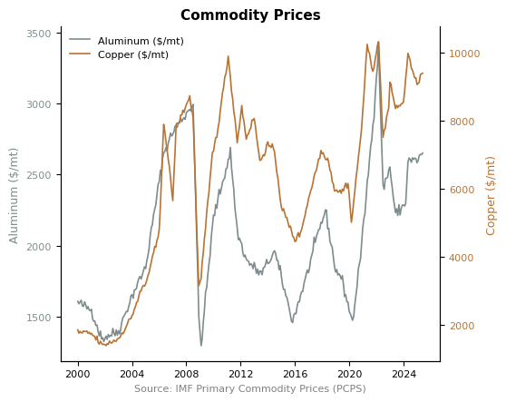
With two metals on different scales (aluminum ~$2,500/mt, copper ~$9,000/mt), a dual-axis chart shows both clearly:
In[7]:
fig, ax1 = plt.subplots()
ax1.plot(df.index, df['Aluminum ($/mt)'],
         color='#7f8c8d', label='Aluminum')
ax1.set_ylabel('Aluminum ($/mt)')

ax2 = ax1.twinx()
ax2.plot(df.index, df['Copper ($/mt)'],
         color='#b87333', label='Copper')
ax2.set_ylabel('Copper ($/mt)')

ax1.set_title('Commodity Prices')
ax1.set_xlabel('Source: IMF Primary Commodity Prices (PCPS)')
lines = ax1.lines + ax2.lines
ax1.legend(lines, [l.get_label() for l in lines],
           loc='upper left', frameon=False)
Out[7]:

Both metals track global industrial activity, but copper's sharper swings reflect its role as a leading economic indicator. Other key commodity codes include PGOLD (gold), POILAPSP (crude oil), PNGAS (natural gas), and PWHEAMT (wheat). Use the codelist methods from Part 2 to browse the full list.
Bulk Download with Requests
For larger downloads—or if you prefer to skip the sdmx1 dependency—the same API accepts plain HTTP requests. Ask for CSV format and you get a pandas-ready response. As covered in Part 2, the URL follows the pattern https://api.imf.org/external/sdmx/3.0/data/dataflow/{agency}/{dataflow}/{version}/{key}.
Here we download the entire WEO dataset from 2020 onward. The wildcard * in the key position requests all countries and indicators:
In[11]:
import requests
import io

url = ("https://api.imf.org/external/sdmx/3.0/data/"
       "dataflow/IMF.RES/WEO/~/*"
       "?c[TIME_PERIOD]=ge:2020-01")

resp = requests.get(url, headers={"Accept": "text/csv"})
df = pd.read_csv(io.StringIO(resp.text), low_memory=False)

print(f"{len(df):,} rows, {df['COUNTRY'].nunique()} countries, "
      f"{df['INDICATOR'].nunique()} indicators")
Out[11]:
86,981 rows, 208 countries, 145 indicators
With the full dataset in memory, filtering is straightforward. For example, G7 real GDP growth:
In[12]:
g7 = ['USA', 'GBR', 'DEU', 'FRA', 'JPN', 'ITA', 'CAN']
gdp = df[df['INDICATOR'] == 'NGDP_RPCH'].copy()
gdp = gdp[gdp['COUNTRY'].isin(g7)]
gdp = gdp.set_index(['TIME_PERIOD', 'COUNTRY'])['OBS_VALUE'].unstack()
gdp.sort_index().round(1)
Out[12]:
COUNTRY  CAN  DEU  FRA   GBR  ITA  JPN  USA
2020    -5.0 -4.1 -7.6 -10.3 -8.9 -4.2 -2.1
2021     6.0  3.9  6.8   8.6  8.9  2.7  6.2
2022     4.2  1.8  2.8   4.8  4.8  1.0  2.5
2023     1.5 -0.9  1.6   0.4  0.7  1.2  2.9
2024     1.6 -0.5  1.1   1.1  0.7  0.1  2.8
2025     1.2  0.2  0.7   1.3  0.5  1.1  2.0
2026     1.5  0.9  0.9   1.3  0.8  0.6  2.1
...
This approach downloads about 8 MB and takes a few seconds. It is useful when you want many indicators or countries at once, or when you want to avoid installing sdmx1. The same pattern works for other dataflows—swap in IMF.STA/CPI for CPI data or IMF.STA/BOP for balance of payments.
Key Concepts
- The discovery methods from Part 2—
dataflow(),dsd.dimensions, and codelist searches—are essential for working with new datasets - WEO provides IMF forecasts, valuable for projections and scenario analysis
- PCPS provides world benchmark commodity prices; the reference area
W00covers all series - The sdmx1 library also supports ECB, BIS, OECD, and many other SDMX providers—run
sdmx.list_sources()to see all of them - For bulk downloads or to avoid dependencies, the API also accepts plain
requestswithAccept: text/csv—see Part 2 for the URL pattern and gotchas - Always call
.sort_index()after converting the time index—SDMX responses are not guaranteed to be in chronological order
Additional Resources
- sdmx1 on PyPI — Installation and basic documentation
- sdmx1 documentation — Full library reference, including the list of supported providers
- IMF Data Portal — Browse available IMF datasets interactively


