Data & PythonTrade & International

Dollar-indices: hitting recent lows (and how to plot with Python)

April 22, 2016 · by Brian Dew

While the dollar has depreciated against most major currencies over the past month (notably 4.4% against the Canadian dollar, 3.3% against the Yen, 4.2% against the Real, and 8.6% against the Rand), the Fed H.10 release provides measures of exactly how much the value of the greenback has fallen relative to a weighted set of its trading partners. The latest data show that the U.S. dollar has fallen on April 12 to its lowest level since June 2015 compared to other major currencies, and its lowest level since October 2015 compared to a broad index of currencies.

This post covers the trade-weighted dollar and is split into two segments: a description of the index and its recent behavior, and a short python script showing how you can use the pandas and matplotlib libraries to retrieve the time series and plot it.

Two trade-weighted dollar indices, described

The Fed’s two most common trade-weighted indices of the foreign exchange value of the U.S. dollar are the major-currencies index and the broad-index. Both measure the value of the dollar relative to other countries’ currencies and intend to be aligned, through their weighting system, with the currencies closely related to U.S. trade patterns. The broad index, however, covers more currencies, and especially more emerging market currencies.

Discrepancies between even the broad index and the way the dollar is actually traded are inevitable. For example, the broad index weight in 2016 for Canada is 12.664 percent (broad index weights are updated yearly), whereas year-t0-date, 15.2 percent of total U.S. trade has been with Canada. From a share-of-total-U.S.-trade perspective, the broad index is somewhat overweight the Yuan, Euro, and Yen, and underweight the Canadian dollar and Mexican peso.

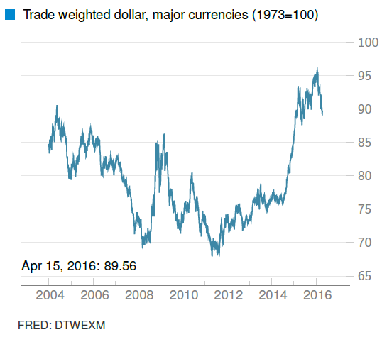The major currencies index contains fewer currencies than the broad index, and has fallen to a 22-month low. (plot from [dashboard](/chartbook.html))

From 2005 through 2015, the major currencies index remained largely within a range of 70-85. After a steep climb through 2015, in January, the measure peaked at 95.8, to the frustration of U.S. exporters whose customers essentially pay more for the same goods (and as a result buy fewer). On April 12, the major currencies index hit its lowest level since June 2015.

Meanwhile, the broad index has moved in the same direction, hitting a five month low on April 12. The plot of the broad index is below, including how to obtain it. You can substitute DTWEXB with DTWEXM if you are interested in the major currencies index.

Python: Retrieve and plot the trade-weighted dollar

Next we show how Python can be used to gather and plot data on the Fed’s broad index of the foreign exchange value of the dollar. The script gathers data from [Fred](https://research.stlouisfed.org/fred2/series/DTWEXM) and plots each business day’s index value since the start of 2014.

### Gathering data First, we import pandas, numpy, and matplotlib and give them conventional short names. We will also use datetime and date.

In \[1\]:

    # Import libraries
    import pandas as pd
    import numpy as np
    import matplotlib as mpl
    import matplotlib.pyplot as plt
    %matplotlib inline
    import datetime
    from datetime import date

Next, we use the pandas.io.data package to request the data from Fred. I’ve found the code for our series of interest, DTWEXB, by searching, but you can also find it on the Fred site by source (Board of Governors of the Federal Reserve System), or by release (H.10). We paste the series code into the datareader and provide start and end dates. Pandas retrieves the data into a dataframe.

In \[2\]:

    import pandas_datareader.data as webdata
    tstart = datetime.datetime(2014, 1, 1)
    #retrieve trade-weighted dollar data from fred
    dtwexb = webdata.DataReader("DTWEXB", "fred", tstart);
    #display five most recent observations
    dtwexb.tail(5)

Out\[2\]:

| | DTWEXB | |------------|----------| | DATE | | | 2016-04-11 | 119.4527 | | 2016-04-12 | 119.2860 | | 2016-04-13 | 119.6278 | | 2016-04-14 | 119.6472 | | 2016-04-15 | 119.6701 |

When was the last time the measure was as low as its April 12 value?

In \[3\]:

print dtwexb[119.29>=dtwexb].dropna().tail(2)

DTWEXB DATE 2015-10-21 119.1786 2016-04-12 119.2860

### Line plot of data Lastly, we can use matplotlib to plot the data.

In \[4\]:

    #Create figure and plot dtwexb
    fig = plt.figure(figsize=[7,5])
    ax1 = plt.subplot(111)
    line = dtwexb.DTWEXB.plot(color='blue',linewidth=2)

    #Add a title
    ax1.set_title('Trade-Weighted U.S. Dollar, Broad Index (1997=100)', fontsize=15)

    #Add y label and no x-label since it is dates
    ax1.set_ylabel('Index')
    ax1.set_xlabel('')

    #Axis options
    ax1.spines["top"].set_visible(False)  
    ax1.spines["right"].set_visible(False)  
    ax1.get_xaxis().tick_bottom()
    ax1.get_yaxis().tick_left()
    ax1.tick_params(axis='x', which='major', labelsize=8)
    ax1.yaxis.grid(True)

    #Annotate with text
    fig.text(0.15, 0.85,'Last: ' + str(dtwexb.DTWEXB[-1]) \
             + ' (as of: ' + str(dtwexb.index[-1].strftime('%Y-%m-%d'))\
             + ')');
    url = 'https://research.stlouisfed.org/fred2/series/TWEXB'
    fig.text(0.05, 0.025, 'Source: ' + url)
    fig.text(0.65, 0.16, 'briandew.wordpress.com')

    #Save as png
    plt.savefig('dtwexb.png', dpi=1000)

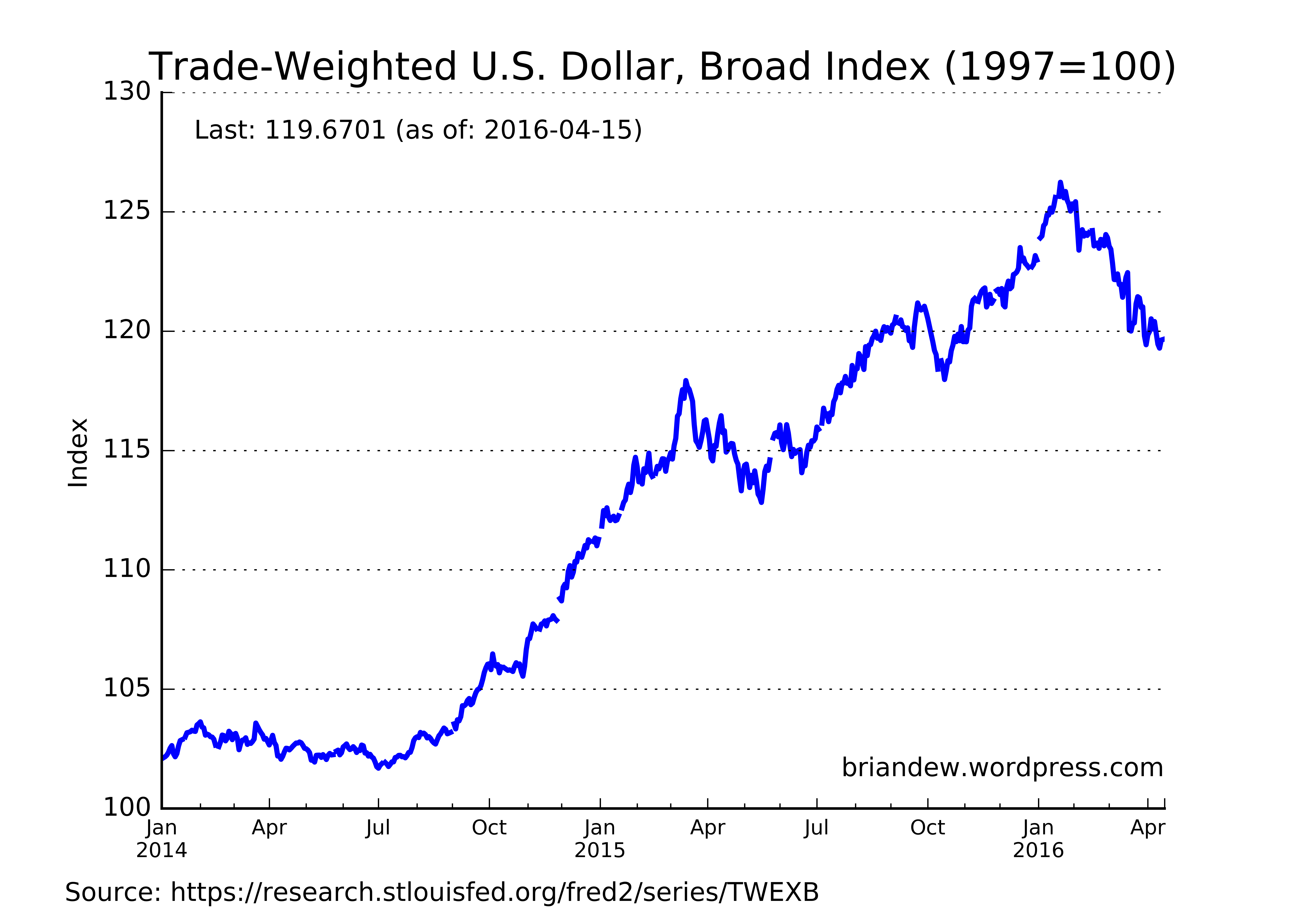The broad index hit a five-month low on April 12.