Data & PythonMacroeconomics
Where Did IFS Go? Accessing IMF Data After the 2025 API Restructuring
Update (2025): The IMF reorganized International Financial Statistics (IFS) data into topic-specific datasets. This post explains the changes and shows how to find former IFS data in the new structure.
For decades, International Financial Statistics (IFS) was the IMF’s flagship macroeconomic database—a one-stop shop for exchange rates, interest rates, prices, production, and national accounts across 180+ countries. If you wrote code against the old IMF API, chances are you pulled from IFS.
In 2025, the IMF restructured its data access around SDMX (Statistical Data and Metadata eXchange) and reorganized IFS into topic-specific datasets. This post explains what changed and shows how to access the same data in the new system.
What Changed
IFS data is now organized around topics, with indicators accessible via specialized datasets. Here are some of the major categories:
| Old IFS Category | New Dataset |
|---|---|
| National Accounts | ANEA (Annual), QNEA (Quarterly) |
| Consumer Prices | CPI |
| Producer Prices | PPI |
| Exchange Rates | ER, EER |
| Interest Rates | MFS_IR |
| Monetary Aggregates | MFS_MA |
| Central Bank Data | MFS_CBS |
| Balance of Payments | BOP |
| International Investment Position | IIP |
| Labor Statistics | LS |
The restructuring reorganized how IFS data is accessed—the same indicators are now distributed across topic-specific datasets. See the official IMF guidance for a complete list.
Finding Former IFS Data
If you have old code that referenced IFS series, there’s no direct lookup from old codes to new ones. The practical approach:
- Identify the category — Determine what type of data you need (prices, interest rates, GDP, etc.) and find the corresponding dataset from the table above.
- Explore the new dataset — Use the IMF Data Portal to browse interactively, or explore codelists programmatically:
import sdmx

IMF_DATA = sdmx.Client('IMF_DATA')

# Example: Find interest rate indicators in MFS_IR
ir_flow = IMF_DATA.dataflow('MFS_IR')
indicators = sdmx.to_pandas(ir_flow.codelist['CL_MFS_IR_INDICATOR'])
print(indicators)
- Verify with IFS_FLAG — Once you’ve found the data, you can confirm it was part of the original IFS by checking the
IFS_FLAGattribute in the returned data:
data_msg = IMF_DATA.data('MFS_IR', key='USA.MFS135_RT_PT_A_PT.M')
df = sdmx.to_pandas(data_msg).reset_index()
print(df['IFS_FLAG'].unique())  # ['true'] confirms this was in IFS
Quick Reference: Retrieving Data
If you already know the dataset and key you need (see the BD Economics IMF API Guide for finding keys), retrieval is straightforward:
import sdmx
import pandas as pd

IMF_DATA = sdmx.Client('IMF_DATA')

# Fetch data
data_msg = IMF_DATA.data('DATASET', key='YOUR.KEY.HERE')
df = sdmx.to_pandas(data_msg).reset_index()
df = df.set_index('TIME_PERIOD')['value']
The sdmx.to_pandas() function returns a Series with a MultiIndex (one level per dimension). Calling .reset_index() converts this to a flat DataFrame with dimensions as columns, which is easier to filter and reshape. The key format varies by dataset—check dimension order with dataflow('DATASET').structure['DSD_...'].dimensions.components. For details on exploring datasets and finding codes, see Part 2 of the BD Economics guide.
Example 1: Banking Spreads Across 80+ Countries
Where the IMF data truly shines is its breadth—comparable data across dozens of countries. For timely data on any single country, you’d go to that country’s central bank. But for cross-country comparisons, the IMF is unmatched.
The MFS_IR dataset contains interest rate data for nearly 100 countries. Let’s compare deposit rates (what banks pay savers) to lending rates (what banks charge borrowers). The spread between them reveals banking sector margins—and varies dramatically across countries.
A few syntax notes for the code below:
- The key format is
COUNTRY.INDICATOR.FREQUENCY—a leading.means “all countries” - Use
+to request multiple codes in one dimension (e.g., two indicators in a single call) - The
paramsdictionary filters by time period
import pandas as pd
import sdmx
import matplotlib.pyplot as plt

IMF_DATA = sdmx.Client('IMF_DATA')

msg = IMF_DATA.data('MFS_IR', key='.MFS135_RT_PT_A_PT+MFS162_RT_PT_A_PT.M',
                    params={'startPeriod': '2023-12', 'endPeriod': '2023-12'})
df = sdmx.to_pandas(msg).reset_index()

# Pivot to wide format: one row per country, indicators as columns
rates = df.pivot(index='COUNTRY', columns='INDICATOR', values='value')
rates.columns = ['deposit_rate', 'lending_rate']
rates = rates.dropna()

# Plot (excluding extreme outliers)
df_plot = rates[(rates['deposit_rate'] < 50) & (rates['lending_rate'] < 60)]

plt.figure(figsize=(7, 5))
plt.scatter(df_plot['deposit_rate'], df_plot['lending_rate'],
            s=50, alpha=0.6, c='steelblue')

# Add 45° line (points on this line have zero spread)
max_val = max(df_plot['deposit_rate'].max(), df_plot['lending_rate'].max())
plt.plot([0, max_val], [0, max_val], 'k--', alpha=0.3, linewidth=1)

plt.xlabel('Deposit Rate (%)')
plt.ylabel('Lending Rate (%)')
plt.title(f'Bank Deposit vs Lending Rates ({len(df_plot)} Economies, Dec 2023)')
plt.grid(True, alpha=0.3)
plt.show()
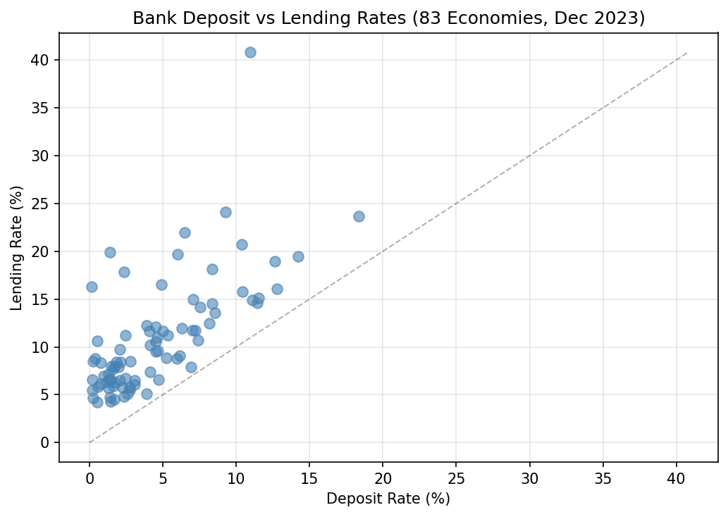
With a single dataset (MFS_IR), we get a global view of banking sector margins. The vertical distance from the 45° line shows the spread—how much more banks charge borrowers than they pay depositors. Brazil stands out with a 30% spread (11% deposit, 41% lending), while developed economies cluster near the bottom with spreads of 2-4%.
Key codes for MFS_IR:
MFS135_RT_PT_A_PT— Deposit rate (% per annum)MFS162_RT_PT_A_PT— Lending rate (% per annum)MFS166_RT_PT_A_PT— Policy/central bank rate (% per annum)
Example 2: Quarterly GDP Growth (QNEA)
The old IFS “National Accounts” data is now split between ANEA (annual) and QNEA (quarterly). QNEA is particularly useful for tracking business cycles and comparing growth across countries.
Let’s compare year-over-year GDP growth for four major emerging markets.
The key format for QNEA is COUNTRY.INDICATOR.PRICE_TYPE.S_ADJUSTMENT.TYPE_OF_TRANSFORMATION.FREQUENCY. In our key:
IND+CHN+BRA+MEX— four countries in one requestB1GQ— GDP indicatorQ— constant prices (real GDP, not nominal)- Empty dimensions (
..) mean “all values”—we’ll filter afterward XDC— domestic currencyQ— quarterly frequency
import pandas as pd
import sdmx
import matplotlib.pyplot as plt

IMF_DATA = sdmx.Client('IMF_DATA')

msg = IMF_DATA.data('QNEA', key='IND+CHN+BRA+MEX.B1GQ.Q..XDC.Q',
                    params={'startPeriod': '2020'})
df = sdmx.to_pandas(msg).reset_index()
df = df[df['S_ADJUSTMENT'] == 'NSA']  # Use NSA for consistency

# Convert quarters to dates and pivot to wide format
df['date'] = pd.PeriodIndex(df['TIME_PERIOD'], freq='Q').to_timestamp()
pivot = df.pivot(index='date', columns='COUNTRY', values='value')

# Calculate year-over-year growth (4 quarters back)
growth = pivot.pct_change(periods=4, fill_method=None) * 100
growth = growth[growth.index >= '2022-07-01']

# Plot
growth.rename(columns={'IND': 'India', 'CHN': 'China', 'BRA': 'Brazil', 'MEX': 'Mexico'}).plot(
    figsize=(5, 5), linewidth=2)
plt.axhline(y=0, color='black', linewidth=0.5)
plt.ylabel('Year-over-Year Growth (%)')
plt.title('Quarterly Real GDP Growth')
plt.grid(True, alpha=0.3)

# Add padding to y-axis so legend doesn't overlap data
ymin, ymax = plt.ylim()
plt.ylim(ymin - (ymax - ymin) * 0.1, ymax + (ymax - ymin) * 0.2)
plt.show()
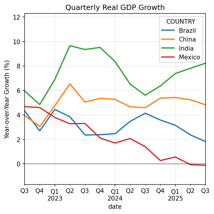
The chart shows how quarterly GDP growth has evolved across these four economies. India consistently posts the strongest growth, while the others show more volatility. This kind of cross-country comparison—using standardized definitions across dozens of economies—is where IMF data is most valuable.
Key codes for QNEA:
B1GQ— Gross Domestic ProductB1G— Gross Value AddedP3— Final Consumption ExpenditureP51G— Gross Fixed Capital FormationP6— Exports of Goods and ServicesP7— Imports of Goods and Services
Price types: V (current prices), Q (constant/real prices), PD (deflator)
Seasonal adjustment: SA (seasonally adjusted), NSA (not adjusted)
Summary
The IFS restructuring means:
- Same data, new organization — Former IFS series are now in topic-specific datasets
- IFS_FLAG identifies legacy data — Check this attribute to find former IFS series
- Key formats vary by dataset — Use
dimensions.componentsto find the order - SDMX is the new standard — The
sdmx1library works with IMF, World Bank, ECB, and OECD
For detailed guidance on exploring datasets and finding codes, see:
- BD Economics IMF API Guide Part 1 — Data retrieval basics
- BD Economics IMF API Guide Part 2 — Finding datasets and codes
Resources
- IMF Data Portal — Browse datasets interactively
- Accessing IFS in the New Portal — Official IMF guidance
- sdmx1 documentation — Full library reference
- sdmx1 on PyPI — Installation