Machine Reading IMF Data: Data Retrieval with Python (2025 Update)

Update (2025): The IMF API has changed significantly. This post has been completely rewritten to use the new SDMX-based API and the sdmx1 Python library, replacing the old JSON REST approach. The underlying data is the same—only the access method has changed.

The IMF’s data portal provides access to macroeconomic data covering more than 180 countries. With Python’s sdmx1 library, retrieving this data programmatically is straightforward.

In this post, I’ll walk through retrieving trade data from the IMF, building up to a comparison of how the United States, China, and Japan’s shares of world exports have shifted over the past 75 years.

Setup

First, install the sdmx1 library:

pip install sdmx1

Step 1: Connect to the IMF API

The IMF provides data through an SDMX endpoint. SDMX (Statistical Data and Metadata eXchange) is a standard format used by many statistical organizations—including the World Bank, ECB, and OECD—so the skills you learn here transfer to other data sources.

We create a client to access the IMF’s endpoint:

import sdmx

IMF_DATA = sdmx.Client('IMF_DATA')

Step 2: Find Available Datasets

The IMF organizes its data into datasets (called “dataflows” in SDMX terminology). The dataflow() method returns all available datasets. We can search for trade-related data:

flows = IMF_DATA.dataflow()

# Search for datasets containing "Trade"
trade_datasets = {k: v.name['en'] for k, v in flows.dataflow.items()
                  if 'Trade' in v.name['en']}

for dataset_id, name in trade_datasets.items():
    print(f"{dataset_id}: {name}")

Output:

ITG: International Trade in Goods (ITG)
ITG_WCA: International Trade in Goods, World and Country Aggregates
IMTS: International Trade in Goods (by partner country) (IMTS)
ITS: International Trade in Services (ITS)
...

The ITG dataset contains country-level export and import values—exactly what we need for our first example.

Step 3: Examine Dataset Structure

Before we can request data, we need to understand how the dataset is organized. Each dataset has dimensions—think of these as columns in a database. Each unique combination of dimension values identifies a specific time series.

itg_flow = IMF_DATA.dataflow('ITG')
dsd = itg_flow.structure['DSD_ITG']

for dim in dsd.dimensions.components:
    print(dim.id)

Output:

COUNTRY
INDICATOR
TYPE_OF_TRANSFORMATION
FREQUENCY
TIME_PERIOD

So to request data from ITG, we need to specify: which country, which indicator, what transformation (units), and what frequency.

Step 4: Find Valid Codes

Each dimension has a codelist defining valid values. Let’s explore what’s available.

For indicators:

# Indicator codes
indicators = sdmx.to_pandas(itg_flow.codelist['CL_ITG_INDICATOR'])
print(indicators)

Output:

MG                       Imports of goods
XG                       Exports of goods
MG_PD    Imports of goods, Price deflator
XG_PD    Exports of goods, Price deflator
...

The transformation codes tell us the units and valuation method:

# Transformation codes
transforms = sdmx.to_pandas(itg_flow.codelist['CL_ITG_TYPE_OF_TRANSFORMATION'])
print(transforms.head(6))

Output:

CIF_XDC       Cost insurance freight (CIF), Domestic currency
FOB_XDC                Free on board (FOB), Domestic currency
CIF_USD               Cost insurance freight (CIF), US dollar
FOB_USD                        Free on board (FOB), US dollar
CIF_USD_IX    Cost insurance freight (CIF), US dollars, index
CIF_IX                    Cost insurance freight (CIF), Index

FOB (Free on Board) is the value at the exporter’s border; CIF (Cost, Insurance, Freight) includes shipping costs to the importer. For exports, FOB is standard.

We can also search for country codes:

countries = sdmx.to_pandas(itg_flow.codelist['CL_COUNTRY'])
countries[countries.str.contains('United States', case=False)]

Output:

USA    United States

Step 5: Construct the Data Request

Now that we know the valid codes, we can construct a “key” to request specific data. The key format for ITG is: COUNTRY.INDICATOR.TRANSFORMATION.FREQUENCY

For US annual exports in US dollars:

key = 'USA.XG.FOB_USD.A'

Breaking this down:

• USA = United States (country code)
• XG = Exports of goods (indicator)
• FOB_USD = Free on board, US dollars (transformation)
• A = Annual (frequency)

Step 6: Retrieve the Data

With our key constructed, we call the .data() method to fetch the data, then use sdmx.to_pandas() to convert it to a familiar pandas DataFrame:

import pandas as pd

usa_msg = IMF_DATA.data('ITG', key='USA.XG.FOB_USD.A')
usa = sdmx.to_pandas(usa_msg).reset_index()
usa = usa.set_index('TIME_PERIOD')['value']

print(f"Retrieved {len(usa)} annual observations")
print(f"Date range: {usa.index.min()} to {usa.index.max()}")

Output:

Retrieved 77 annual observations
Date range: 1948 to 2024

Step 7: Prepare for Analysis

The data comes with string time periods (like “2024”). We convert the index to proper datetime objects for plotting, and scale the values to billions for readability:

df = pd.DataFrame({'US_Exports': usa})
df.index = pd.to_datetime(df.index, format='%Y')
df = df.sort_index()

# Convert to billions for readability
df['US_Exports_Billions'] = df['US_Exports'] / 1e9

Step 8: Visualize

With the data in hand, we can create a simple visualization:

import matplotlib.pyplot as plt

fig, ax = plt.subplots(figsize=(6, 3.5))
df['US_Exports_Billions'].plot(ax=ax, color='dodgerblue', linewidth=2.5)
ax.set_title('US Goods Exports')
ax.set_ylabel('Billions USD')
ax.grid(True, alpha=0.3)
plt.show()

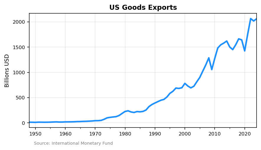
US goods exports have grown from under $15 billion in 1948 to over $2 trillion today.

Step 9: Combining Datasets for Comparative Analysis

So far we’ve worked with a single dataset. But real-world analysis often requires combining data from multiple sources.

To calculate each country’s share of world exports, we need world totals. The ITG dataset has country-level data, but world aggregates live in the IMTS dataset (International Trade in Goods by partner country). IMTS includes aggregate trade flows using G001 (World) as both the reporting country and counterpart. This separation is common in statistical APIs—different datasets serve different purposes.

You can request multiple countries in a single call by joining codes with +:

# Country data from ITG (all three countries in one request)
countries_msg = IMF_DATA.data('ITG', key='USA+CHN+JPN.XG.FOB_USD.A')
countries_df = sdmx.to_pandas(countries_msg).reset_index()
countries_df = countries_df.set_index(['TIME_PERIOD', 'COUNTRY'])['value'].unstack()
countries_df = countries_df.rename(columns={'USA': 'United States', 'CHN': 'China', 'JPN': 'Japan'})

# World totals from IMTS (G001 = World, for both reporter and partner)
world_msg = IMF_DATA.data('IMTS', key='G001.XG_FOB_USD.G001.A')
world_annual = sdmx.to_pandas(world_msg).reset_index()
world_annual = world_annual.set_index('TIME_PERIOD')['value']

Combine and calculate shares:

df_annual = countries_df.copy()
df_annual['World'] = world_annual
df_annual.index = pd.to_datetime(df_annual.index, format='%Y')

shares = df_annual[['United States', 'China', 'Japan']].div(df_annual['World'], axis=0) * 100
shares_ma = shares.rolling(3).mean().dropna()

Step 10: The Big Picture

Finally, we can visualize how global trade has shifted over 75 years:

fig, ax = plt.subplots(figsize=(6, 3.5))

colors = {'United States': 'dodgerblue', 'China': 'crimson', 'Japan': 'darkorange'}
for country, color in colors.items():
    shares_ma[country].plot(ax=ax, color=color, linewidth=2.5, label=country)

ax.set_title('Share of World Goods Exports')
ax.set_ylabel('Percent')
ax.legend(loc='upper right')
ax.grid(True, alpha=0.3)
plt.show()

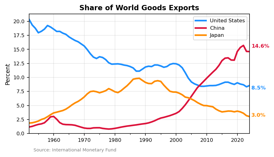
The chart reveals the dramatic shift in global trade over 75 years:

• United States declined from ~20% of world exports in 1950 to 8.5% today
• China rose from near zero to 14.6%, surpassing the US around 2007
• Japan peaked at ~10% during its 1980s boom, then fell to 3%

Step 11: Export to CSV

To make the data available for use in other tools—Excel, R, or any application that reads CSV files:

shares.to_csv('export_share_data.csv')

Summary

The workflow for accessing IMF data:

1. Connect: sdmx.Client('IMF_DATA')
2. Find datasets: dataflow() and search by name
3. Get structure: Check dimensions.components for the key format
4. Find codes: Use codelist to look up valid values
5. Build key: Join dimension values with dots (e.g., USA.XG.FOB_USD.A)
6. Retrieve: .data('DATASET', key='...')
7. Convert: sdmx.to_pandas() for analysis

Next Steps

Part 2 covers where former IFS data now lives after the 2025 restructuring, with examples using the new topic-specific datasets.

Resources

• sdmx1 on PyPI – Installation and documentation
• sdmx1 documentation – Full library reference
• IMF Data Portal – Browse datasets interactively
• BD Economics IMF API Guide – Extended version with additional examples